How do I freeze a row in Excel?

To freeze rows:

1. Select the row below the row(s) you want to freeze. In our example, we want to freeze rows 1 and 2, so we'll select row 3.
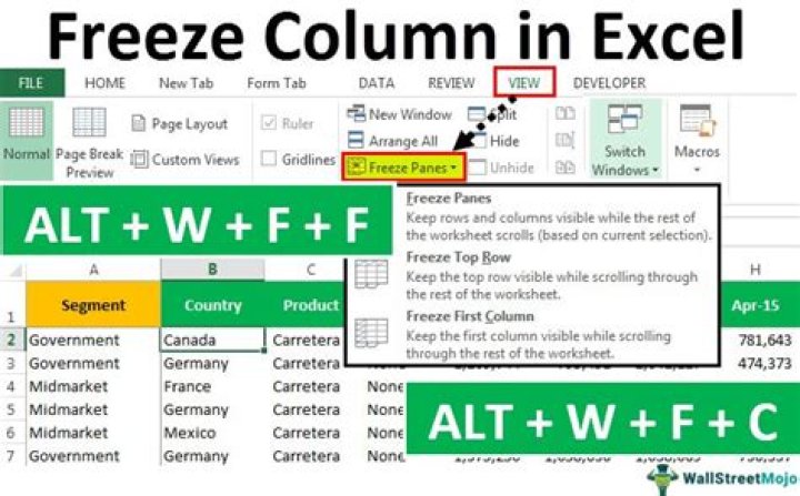
2. Click the View tab on the Ribbon.
3. Select the Freeze Panes command, then choose Freeze Panes from the drop-down menu.
4. The rows will be frozen in place, as indicated by the gray line.

.

Regarding this, how do I freeze multiple rows and columns in Excel?

To lock multiple rows (starting with row 1), select the row below the last row you want frozen, choose the View tab, and then click Freeze Panes. To lock multiple columns, select the column to the right of the last column you want frozen, choose the View tab, and then click Freeze Panes.

how do I freeze a row in Excel on a Mac? To freeze the top row, open your Excel spreadsheet. Select the Layout tab from the toolbar at the top of the screen. Click on the Freeze Panes button and click on the Freeze Top Row option in the popup menu. Now when you scroll down, you should still continue to see the column headings.

Subsequently, one may also ask, how do I freeze a column in Excel?

How to Freeze Rows in Excel

1. How to Freeze Rows in Excel.
2. Select the row right below the row or rows you want to freeze. If you want to freeze columns, select the cell immediately to the right of the column you want to freeze.
3. Go to the View tab.
4. Select the Freeze Panes command and choose "Freeze Panes."

How do I freeze a row in Excel 2007?

To freeze the first row and column, open your Excel spreadsheet. Select cell B2. Then select the View tab from the toolbar at the top of the screen and click on the Freeze Panes button in the Window group. Then click on the Freeze Panes option in the popup menu.

Related Question Answers

How do I freeze multiple rows in Excel 2019?

Freezing Columns and Rows

1. To freeze a set of columns and rows at the same time, click on the cell below and to the right of the panes you want to freeze.
2. With the proper cell selected, select the “View” tab at the top and click on the “Freeze Panes” button, and select the “Freeze Panes” option in the drop-down.

How do I freeze rows and columns?

Freeze columns and rows

1. Select the cell below the rows and to the right of the columns you want to keep visible when you scroll.
2. Select View > Freeze Panes > Freeze Panes.

How do I freeze multiple rows in Excel 365?

Freeze columns and rows to keep them in view while you scroll through your data.

1. Select the cell below the rows, and to the right of the columns you want to freeze.
2. Click View > Freeze Panes > Freeze Panes.

Can you lock cells in Excel?

Follow these steps to lock cells in a worksheet: Select the cells you want to lock. On the Home tab, in the Alignment group, click the small arrow to open the Format Cells popup window. On the Protection tab, select the Locked check box, and then click OK to close the popup.

How do I freeze rows and columns at the same time in Excel 2010?

To freeze the first row and column, open your Excel spreadsheet. Select cell B2. Then select the View tab from the toolbar at the top of the screen and click on the Freeze Panes button in the Window group. Then click on the Freeze Panes option in the popup menu.

Why can't I freeze panes in Excel?

To enable the Freeze Panes command again, you must choose either the Normal or Page Break Preview commands. You'll have to manually restore any frozen panes that you lost when you chose Page Layout view. Figure 1: Excel's Page Layout command disables the Freeze Panes command and unfreezes rows/columns, as well.

How do I freeze panes in Excel 2010?

To freeze rows:

1. Select the row below the rows you want frozen. For example, if you want rows 1 and 2 to always appear at the top of the worksheet even as you scroll, then select row 3.
2. Click the View tab.
3. Click the Freeze Panes command.
4. Select Freeze Panes.
5. A black line appears below the rows that are frozen in place.

How do I freeze rows and columns at the same time in Excel 2003?

To freeze the first row and column, open your Excel spreadsheet. Select cell B2. Then under the Window menu, select Freeze Panes. Now when you scroll, you should still continue to see row 1 and column A.

How do you keep a cell fixed in Excel?

Keep formula cell reference constant with the F4 key 1. Select the cell with the formula you want to make it constant. 2. In the Formula Bar, put the cursor in the cell which you want to make it constant, then press the F4 key.

How do I make a floating header in Excel?

Here is how you do it:

1. This moment is the key - select the cell just below the rows you want to freeze, and to the right of such columns if needed.
2. Open the View tab in Excel and find the Freeze Panes option in the Window group.
3. Click on the little arrow next to it to see all the options, and choose to Freeze Panes.

How do you lock rows when filtering?

How to lock multiple Excel rows

1. Start by selecting the row below the last row you want to freeze. For example, if you wish to lock the top two rows, place the mouse cursor in cell A3 or select the entire row 3.
2. Head over to the View tab and click Freeze Panes > Freeze Panes.

How do I make the first row in Excel a header?

Go to the "Insert" tab on the Excel toolbar, and then click the “Header & Footer” button in the Text group to start the process of adding a header. Excel changes the document view to a Page Layout view. Click on the top of your document where it says “Click to Add Header,” and then type the header for your document.

What is the shortcut to freeze panes in Excel 2007?

Freeze panes: Put the active cell in the desired location, and press Alt+w and then F. To remove the freeze panes, use the same shortcut.

How do I freeze a filter in Excel?

Select the column to the right of the columns you want to freeze, or row beneath the rows to freeze. Click on the Window menu, and then click on the Freeze Panes command.

How do I freeze horizontal and vertical panes in Excel?

To freeze horizontal and vertical headings simultaneously:

1. Select the cell in the upper-left corner of the range you want to remain scrollable.
2. Select View tab, Windows Group, click Freeze Panes from the menu bar.
3. Excel inserts two lines to indicate where the frozen panes begin.

How do I lock a column in Excel 2007?

Right-click and then select "Format Cells" from the popup menu. When the Format Cells window appears, select the Protection tab. Check the "Locked" checkbox. Click the OK button.

How do I freeze multiple rows and columns at the same time in Excel 2007?

To lock multiple rows (starting with row 1), select the row below the last row you want frozen, choose the View tab, and then click Freeze Panes. To lock multiple columns, select the column to the right of the last column you want frozen, choose the View tab, and then click Freeze Panes.

Can you freeze both rows and columns in Excel?

Besides locking columns and rows separately, Microsoft Excel lets you freeze both rows and columns at the same time. Here's how: Select a cell below the last row and to the right of the last column you'd like to freeze. On the View tab, click Freeze Panes > Freeze Panes.