How do you make a graph with two y axis in Google Sheets?

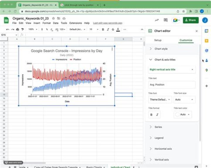
Add a second Y-axis

1. On your computer, open a spreadsheet in Google Sheets.
2. Double-click the chart you want to change.
3. At the right, click Customize.
4. Click Series.
5. Optional: Next to "Apply to," choose the data series you want to appear on the right axis.
6. Under "Axis," choose Right axis.

.

Also know, how do you make a graph with two y axis?

Add a secondary horizontal axis (Office 2010)

1. Click a chart that displays a secondary vertical axis. This displays the Chart Tools, adding the Design, Layout, and Format tabs.
2. On the Layout tab, in the Axes group, click Axes.
3. Click Secondary Horizontal Axis, and then click the display option that you want.

how do I combine two graphs in Google Sheets? 2. Charts with Two Y-Axes

1. Highlight to sets of data you want to chart together.
2. Click “Insert”>”Chart” on the menu.
3. Select the chart type and click “Insert”
4. Right click your new chart and select “Series”>”Series you want to move to the right axis” (that's not really what is says, by the way)

Likewise, people ask, how do I reverse the y axis in Google Sheets?

2 Answers

1. Make a new column, make it equal to zero minus your data column for the vertical axis.
2. Replace the data column address in the chart with this new column.
3. Select the column.
4. Click format>number>more formats>custom number format.

What is a double Y axis graph?

If two columns of values are selected (or a range of two columns), then one data plot displays in each layer. Each data point in the data plot is connected by a line. The default line connection between points is a straight line. The data points are displayed as symbols.

Related Question Answers

What is a secondary axis?

Definition of secondary axis. : a line through the center of a thin lens or through the center of curvature of a concave or convex mirror other than the principal axis of the lens or mirror.

What is a dual axis chart?

A dual axis chart is a great way to easily illustrate the relationship between two different variables. They illustrate a lot of information with limited space and allow you to discover trends you may have otherwise missed if you're switching between graphs.

How do you format an axis in Excel?

1. Click anywhere in the chart. This displays the Chart Tools, adding the Design, Layout, and Format tabs.
2. On the Format tab, in the Current Selection group, click the arrow in the Chart Elements box, and then click the axis that you want to select.

Can you have 3 y axis Excel chart?

There is a way of displaying 3 Y axis see here. Excel supports Secondary Axis, i.e. only 2 Y axis. Other way would be to chart the 3rd one separately, and overlay on top of the main chart. An alternative is to normalize the data.

How do you flip Y axis?

Flipping axis using the Format Axis dialog The first thing we have to flip x and y axis is to select the Format Axis button. To do this, we have to right click the y axis that we want to reverse. Then, select the Format Axis from the context menu. The next thing to do is to check the Categories in reverse order.

How do you graph on Google Sheets?

How to Make a Graph or Chart in Google Sheets

1. Click Insert.
2. Select Chart.
3. Select a kind of chart. Pie charts are best for when all of the data adds up to 100 percent, and histograms work best for data compared over time.
4. Click Chart Types for options including switching what appears in the rows and columns or other kinds of graphs.
5. Click Insert.

What does aggregate mean in Google Sheets?

Aggregation. The method used to summarize data. In general data science terms, an aggregation is "a function or field where the values of multiple rows are grouped together as input on certain criteria to form a single value of more significant meaning or measurement." (

How do I add axis labels in Excel?

Click the chart, and then click the Chart Layout tab. Under Labels, click Axis Titles, point to the axis that you want to add titles to, and then click the option that you want. Select the text in the Axis Title box, and then type an axis title.

How do I invert a graph in Excel?

Rotating the Excel chart

1. Click on the chart to see Chart Tools on the Ribbon.
2. Select the Format tab.
3. Go to the Chart Elements drop down list and pick Vertical (Value) Axis.
4. Click the Format Selection button to see the Format Axis window.
5. On the Format Axis window tick the Values in reverse order checkbox.

How do you add a trendline in Google Sheets?

To add a trendline:

1. Open Google Sheets.
2. Open a spreadsheet with a chart where you want to add a trendline.
3. Select the chart and in the top right corner, click the drop-down arrow.
4. Select Advanced edit.
5. Click the Customize tab and scroll to the “Trendline” section at the bottom.
6. The trendline is set to “None” by default.

What is compare mode in Google Sheets?

The compare mode type, which describes the behavior of tooltips and data highlighting when hovering on data and chart area.

How do you combine two bar graphs?

Select the two sets of data you want to use to create the graph. Choose the "Insert" tab, and then select "Recommended Charts" in the Charts group. Select "All Charts," choose "Combo" as the chart type, and then select "Clustered Column - Line," which is the default subtype.

How do I compare two data sets in Google Sheets?

Compare two columns in Google Sheets

1. Open your Sheet on the page that you want to compare.
2. With data in columns A and B, highlight cell C1.
3. Paste '=if(A1=B1,“”,“Mismatch”)' into cell C1.
4. Left-click on the bottom right corner of cell C1 and drag downwards.

How do you combine a line and bar graph?

Combination Chart

1. On the Insert tab, in the Charts group, click the Combo symbol.
2. Click Create Custom Combo Chart.
3. The Insert Chart dialog box appears. For the Rainy Days series, choose Clustered Column as the chart type. For the Profit series, choose Line as the chart type.
4. Click OK. Result:

How do I use Google charts?

The most common way to use Google Charts is with simple JavaScript that you embed in your web page. You load some Google Chart libraries, list the data to be charted, select options to customize your chart, and finally create a chart object with an id that you choose.

How do you add a line in a graph?

In the chart, select the data series that you want to add a line to, and then click the Chart Design tab. For example, in a line chart, click one of the lines in the chart, and all the data marker of that data series become selected. Click Add Chart Element, and then click Gridlines.

Which one is a compound graph?

Compound graphs include more than one graph positioned in the same display. Certain types of Graphs menu graphs that display different graph types on a single graph, such as scatterplots with box plots, scatterplots with histograms, and matrix plots.

What is a compound bar graph?

A compound bar chart is a graph which combines two or more types of information in one chart. A compound bar chart is a type of bar chart where columns can be split into sections to show breakdown of data.